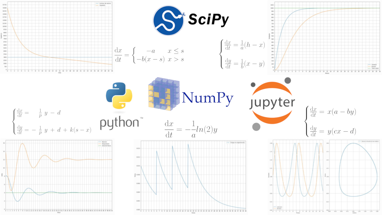
Ordinary Differential Equations (ODE) with Python

29 Jan 2019

18 min to read

When I was at my 3rd year of University I have a complete subject about Ordinary Differential Equations and other similar topics. For that course we used Wolfram Mathematica throughout the year and I asked the teacher whether I can do it with Python, here you can see the results.

Of course in one year one solves a lot of differential equations but there were some problems that I think are really interesting and that rely on ordinary differential equations (ODE), numerical integration and reasoning. The year after, when I was in my 4th year, I had a subject called simulation where I learnt other techniques with another software and the focus was the process instead of the analytical form.

The teacher showed us several situations one can model with ODE and each has its particularities:

Economy of a Home: Piecewise Defined Derivatives
Sales of Houses and Air Conditionings: Systems of ODEs
Stock Control: Systems with oscillation (Underdamped, critically damped, overdamped and undamped)
Useful life in medicine: Start from a previous result
Predator and Prey Model: Non-linear relationships between variables

Some of them are quite well-known but the aim of this post isn't introducing these models but rather how you can solve them with Python, I will also attach the interactive widgets so you can experiment with the models and see how they behave when you change the parameters. Also, I prepared a jupyter notebook where all these models are together, you can open it online and experiment directly. Additionally if you find any of the widgets useful you can embed them in your own website, at the end of each widget the code for doing so will be provided.

This post will have some explanation of the models, and the equations, I won't focused on how to solve a ODE by hand since the focus is the computational aid one can have from open source tools.

Requirements:

Jupyter: Notebook Interface
Numpy: For array manipulation
Scipy: For numerical integration
Matplotlib: For visualization and animation

Imports and setup

Before starting with the models themselves, we need to import some libraries, the imports are the same for all models so one can simply place this snippet at the top of the script/notebook. In this snipped the style for the sliders is also included in order to have the same look and feel in all the widgets

# General Purpose
import numpy as np
from matplotlib import pyplot as plt
from scipy.integrate import odeint

# Jupyter Specifics
from IPython.display import HTML
from ipywidgets.widgets import interact, IntSlider, FloatSlider, Layout

%matplotlib inline

style = {'description_width': '150px'}
slider_layout = Layout(width='99%')

Economy of a Home

A home economy (family) has a fixed income at the beginning of some periodic interval (usually a month), there are also two kind of outcomes, fixed costs and extraordinary expenses, which are proportional to the money at the moment. Additionally, the family decides to set apart some proportion of the income just for fixed costs. This way, when the capital of the family is below this amount, the extraordinary expenses are 0.

The model has the following variables:

initial_salary [$]: the amount of money for the income
savings_ratio [%]: Proportion of the income that will be the keep just for fixed costs
fixed_costs [$]: The amount of money of fixed costs distributed per day
extraordinary_expenses [%]: Proportion of money that will be spend in extraordinary expenses.
days [days]: The time interval until the next income

Notation for the equation:

$x(t):$ Capital over time
$x(0) =$ initial_salary
$s =$ savings_ration * initial_salary
$a =$ fixed_costs
$b =$ extraordinary_expenses

With the previously defined notation, the ordinary differential equation is as follows:

$$ \frac{\mathrm{d} x}{\mathrm{d} t} = \left\{\begin{matrix} - a & x \leq s \\ - b (x - s) & x > s \end{matrix}\right. $$

Below is the resulting model in action and then the code explain part by part.

If you want to embed this widget in your blog/website, just add the following HTML:

<iframe src="https://elc.github.io/blog/iframes/ode-python/home-economy-iframe.html"></iframe>

Code

Now I will comment part by part the code used, at the end of this section, I will place the full code for easy copy/paste

Function Definition

def main(initial_salary, savings_ratio, extraordinary_expenses, fixed_costs, days):

First, we defined a function called main for easier use of interact which will produce the interactive widget. After that, all the constants are calculated, in this case saving_limit which is analogous to $s$ in the equation.

ODE Specifics

saving_limit = savings_ratio * initial_salary

def function(capital, time):
    if capital <= saving_limit:
        out_rate = 0
    else:
        out_rate = extraordinary_expenses * (capital - saving_limit)
    return -fixed_costs - out_rate

time = np.linspace(0, days, days * 10)

solution = odeint(function, initial_salary, time)

A nested function is defined (there could be better ways to do this but I find this the simplest), this function is the differential equation, it should take two parameters and return the value of $\frac{\mathrm{d} x}{\mathrm{d} t}$. The first parameter can be used as the current value of $x$ for a given $t$. For the numerical integration scipy.integrate.odeint is used and that's why this format is required. Using a nested function has the advantage that its name doesn't conflict with the outer scope of the function containing it and that it has access to all the parameters the outer function has, avoiding unnecessary indirection due to reference (If you know a better way to implement this, let me know in the comments).

Then the time variable is defined and initialized, this will be the $t$ steps. We have basically two options here:

Define the start, the end and the number of steps: For this numpy.linspace could be used
Define the start, the end and the step: For this numpy.arange could be used

Note: It is important to note that this will determined how smooth the resulting function will be. Although at first it might seem that the integration step (usually denoted with $h$) is implicitly defined here, that's not the case since, as you can see in the docs of scipy.integrate.odeint, $h$ is determined by the solver in each iteration.

Then the scipy.integrate.odeint function is called with the function defined as a first parameter, the initial conditions as the second and the window time as the third. This function returns the solution array which will be later used for the plotting.

Graphics Specifics

fig, ax = plt.subplots(figsize=(15, 10))

ax.plot((0, days), (saving_limit, saving_limit), label='Saving Limit')
ax.plot(time, solution, label='Capital(t)')

if days <= 60:
    step = 1
    rotation = "horizontal"
elif days <= 300:
    step = 5
    rotation = "vertical"
else:
    step = 10
    rotation = "vertical"

ax.set_xticklabels(np.arange(0, days + 1, step, dtype=np.int), rotation=rotation)
ax.set_xticks(np.arange(0, days + 1, step))

ax.set_yticks(np.arange(0, initial_salary * 1.1, initial_salary / 20))

ax.set_xlim([0, days])
ax.set_ylim([0, initial_salary * 1.1])
ax.set_xlabel('Days')
ax.set_ylabel('Capital $')
ax.legend(loc='best')
ax.grid()

plt.show()

Next, the graphics part, here matplotlib is used and this snipped is specific to this library but I will explain it in order to be self-contained (although I might produce a matplotlib tutorial in the future).

Note: I know there are plenty of plotting libraries, and many even more elegant and powerful than matplotlib but for this use case, where the complexity lies in the differential equation and not in the graphic itself, I believe it is more than enough. For complex graphics such as statistics or big data, I would recommend another library such as bqplot.

First we define a figure and an axes object, explicitly initializing the figure size through figsize. Then a horizontal line with the label Saving Limit is plot at the heigh of the saving_limit and after that the solution is plot with the label Capital(t).

The if-elif-else structure defines how many sticks there will be in the x-axis and if they should be place horizontal or vertically. Then the said sticks are plotted, the same occurs with the yticks. Then the limits for each axis and the labels for each axis are set and finally, the legend position is defined and the grid is added.

Then when plt.show() is called the figure is generated and showed in the screen.

Interaction Specifics

interact(main, initial_salary=IntSlider(min=0, max=25000, step=500, value=15000, description='Initial Salary', style=style, layout=slider_layout),
               savings_ration=FloatSlider(min=0, max=1, step=0.01, value=0.2, description='Savings Ratio', style=style, layout=slider_layout),
               extraordinary_expenses=FloatSlider(min=0, max=1, step=0.005, description='Extraordinary Expenses', style=style, value=0.3, layout=slider_layout),
               fixed_costs=IntSlider(min=1, max=1000, step=1, value=100, description='Fixed Costs', style=style, layout=slider_layout),
               days=IntSlider(min=1, max=600, step=5, value=30, description='Total Number of Days', style=style, layout=slider_layout)
        );

Finally, the code for the interaction, here the interact function from ipywidgets is used. A separate slider is used for each parameter with the default parameters set for a nice default visualization, with a description and the style and layout is used from the initialization cells.

Full code

def main(initial_salary, savings_ratio, extraordinary_expenses, fixed_costs, days):
    saving_limit = savings_ratio * initial_salary

    def function(capital, time):
        if capital <= saving_limit:
            out_rate = 0
        else:
            out_rate = extraordinary_expenses * (capital - saving_limit)
        return -fixed_costs - out_rate

    time = np.linspace(0, days, days * 10)

    solution = odeint(function, initial_salary, time)

    #Graphic details
    fig, ax = plt.subplots(figsize=(15, 10))

    ax.plot((0, days), (saving_limit, saving_limit), label='Saving Limit')
    ax.plot(time, solution, label='Capital(t)')

    if days <= 60:
        step = 1
        rotation = "horizontal"
    elif days <= 300:
        step = 5
        rotation = "vertical"
    else:
        step = 10
        rotation = "vertical"

    ax.set_xticklabels(np.arange(0, days + 1, step, dtype=np.int), rotation=rotation)
    ax.set_xticks(np.arange(0, days + 1, step))

    ax.set_yticks(np.arange(0, initial_salary * 1.1, initial_salary / 20))

    ax.set_xlim([0, days])
    ax.set_ylim([0, initial_salary * 1.1])
    ax.set_xlabel('Days')
    ax.set_ylabel('Capital $')
    ax.legend(loc='best')
    ax.grid()

    plt.show()

interact(main, initial_salary=IntSlider(min=0, max=25000, step=500, value=15000, description='Initial Salary', style=style, layout=slider_layout),
               savings_ratio=FloatSlider(min=0, max=1, step=0.01, value=0.2, description='Savings Ratio', style=style, layout=slider_layout),
               extraordinary_expenses=FloatSlider(min=0, max=1, step=0.005, description='Extraordinary Expenses', style=style, value=0.3, layout=slider_layout),
               fixed_costs=IntSlider(min=1, max=1000, step=1, value=100, description='Fixed Costs', style=style, layout=slider_layout),
               days=IntSlider(min=1, max=600, step=5, value=30, description='Total Number of Days', style=style, layout=slider_layout)
        );

Sales of Houses and Air Conditionings

In a city there are houses and air conditionings (AC) for sale and it's known that these are complementary goods, which means that if the sales of one increase the sales of the other will also increase. The number of houses sales is proportional to the number of houses that weren't sold yet and the number of AC sales is proportional to the houses sold that doesn't yet have an AC.

The model has the following variables:

initial_houses [houses]: Number of Houses initially sold, could be 0.
initial_ac [AC]: Number of air conditionings sold, could be 0 and should be less than initial_houses.
avg_time_house [days]: Average number of days to sell a house.
avg_time_ac [days]: Average number of days to sell an AC.
total_houses [houses]: Total number of Houses for sale.
days [days]: The time interval until the next income

Notation for the equation:

$x(t):$ Number of sold Houses
$y(t):$ Number of sold Air Conditionings
$x(0) =$ initial_houses
$y(0) =$ initial_ac
$h =$ total_houses
$a =$ avg_time_house
$b =$ avg_time_ac

With the previously defined notation, the ordinary differential equation is as follows:

$$ \left\{\begin{matrix} \frac{\mathrm{d} x}{\mathrm{d} t} =\frac{1}{a} (h - x) \\\\ \frac{\mathrm{d} y}{\mathrm{d} t} =\frac{1}{b} (x - y) \end{matrix}\right. $$

Note: The last scenario was a first-order differential equation and in this case it a system of two first-order differential equations, the package we are using, scipy.integrate.odeint can only integrate first-order differential equations but this doesn't limit the number of problems one can solve with it since any ODE of order greater than one can be [and usually is] rewritten as system of first order ODEs ¹

Widget

Embed this widget in your website:

<iframe src="https://elc.github.io/blog/iframes/ode-python/houses-air_conditioning-iframe.html"></iframe>

Code

In this scenario and the followings the code will be explain where it differs from the first example to avoid unnecesary repetition

ODE Specifics

def function(s, time):
    x, y = s
    dydt = [
        (1 / avg_time_house) * (total_houses - x),    # dx/dt: Change in the House sales
        (1 / avg_time_ac)    * (x - y)                # dx/dt: Change in the AC sales
    ]
    return dydt

time = np.linspace(0, days, days * 10)
initial_conditions = [initial_houses, initial_ac]
solution = odeint(function, initial_conditions, time)

In this case the constants avg_time_house and avg_time_ac are used directly inside the function since it is much clearer this way. To define a system of ODEs, first the initial condition should be a list, each element of the list represents the initial condition for each of the variables. The nested function also changes a bit, in order to work, the first parameter would also be a list so it is necessary to unpack it into the variables and then a variable dydt is used (the dydt name doesn't refer to the variable y but rather is the convention in scipy) to represent the system where each element is the left side of each equation (in canonical form).

Although it may differ from PEP8 (Python style for coding), I prefer to split the elements one per line to improve readability. Finally the dydt variable is returned. The definition of time is the same as previously seen and the solution variable is now a nested array containing the solution for both variables. This is specially useful when plotting.

Graphics Specifics

ax.plot(time, solution[:, 0], label='Houses(t)')
ax.plot(time, solution[:, 1], label='Air Conditionings(t)')

These are the only lines that differ in which instead of plotting the solution variable, the numpy indexing and slicing syntax is used to easily split the results from each of the variables.

Full code

def main(initial_houses, initial_ac, avg_time_house, avg_time_ac, total_houses, days):

    def function(s, time):
        x, y = s
        dydt = [
            (1 / avg_time_house) * (total_houses - x), # dx/dt: Change in the House sales
            (1 / avg_time_ac)    * (x - y)             # dx/dt: Change in the AC sales
        ]
        return dydt

    time = np.linspace(0, days, days * 10)
    initial_conditions = [initial_houses, initial_ac]
    solution = odeint(function, initial_conditions, time)

    #Graphic details
    fig, ax = plt.subplots(figsize=(15, 10))

    ax.plot(time, solution[:, 0], label='Houses(t)')
    ax.plot(time, solution[:, 1], label='Air Conditionings(t)')
    ax.plot((0, days), (total_houses, total_houses), label='Total Houses')

    if days <= 60:
        step = 1
        rotation = "horizontal"
    elif days <= 300:
        step = 5
        rotation = "vertical"
    else:
        step = 10
        rotation = "vertical"

    ax.set_xticklabels(np.arange(0, days + 1, step, dtype=np.int), rotation=rotation)
    ax.set_xticks(np.arange(0, days + 1, step))

    ax.set_yticks(np.arange(0, total_houses * 1.1, total_houses / 20))

    ax.set_xlim([0, days])
    ax.set_ylim([0, total_houses * 1.1])
    ax.set_xlabel('Months')
    ax.set_ylabel('Units')
    ax.legend(loc='best')
    ax.grid()

    plt.show()

interact(main, initial_houses=IntSlider(min=0, max=2000, step=10, value=0, description='Initial sold Houses', style=style, layout=slider_layout),
               initial_ac=IntSlider(min=0, max=2000, step=10, value=0, description='Initial sold AC', style=style, layout=slider_layout),
               total_houses=IntSlider(min=1, max=2000, step=100, value=1000, description='Total Houses', style=style, layout=slider_layout),
               avg_time_house=FloatSlider(min=0.1, max=24, step=0.1, value=2, description='Time for House', style=style, layout=slider_layout),
               avg_time_ac=FloatSlider(min=0.1, max=24, step=0.1, value=4, description='Time for AC', style=style, layout=slider_layout),
               days=IntSlider(min=1, max=360, step=10, value=30, description='Total Number of Days', style=style, layout=slider_layout),
        );

Stock Control

A company wants a desired stock, they started with an initial stock and they work with a provider which sends deliveries goods through sales orders. The company asks the provider each day a sales order proportional to the missing or surplus quantity to the desired stock and the market demand. The provider deliver the goods according to the sales order with a constant delay. Finally, the market demand is consider constant. The company wants to know how their stock and their request to the provider will behave and they will try to avoid alternating behavior (oscillation in stock).

The model has the following variables:

desired_stock [goods]: Amount of stock the company wants to have.
initial_stock [goods]: The initial amount of stock of the company.
initial_orders [goods]: initial amount of goods asked in sales orders.
stock_control [%]: Proportion of the missing/surplus stock to ask to the provider.
market_demand [goods]: The daily demand of the market
provider_delay [days]: The number of days of the provider delay.
days [days]: The total number of days the model will analyse.

Notation for the equation:

$x(t):$ Number of goods in stock
$y(t):$ Number of pending sales order sent to the provider
$x(0) =$ initial_stock
$y(0) =$ initial_orders
$s =$ desired_stock
$d =$ market_demand
$k =$ stock_control
$p =$ provider_delay

With the previously defined notation, the ordinary differential equation is as follows:

$$ \left\{\begin{matrix} \frac{\mathrm{d} x}{\mathrm{d} t} =& \frac{1}{p} y - d \\\\ \frac{\mathrm{d} y}{\mathrm{d} t} =& - \frac{1}{p} y + d + k ( s - x ) \end{matrix}\right. $$

Widget

Embed this widget in your website:

<iframe src="https://elc.github.io/blog/iframes/ode-python/stock-control-iframe.html"></iframe>

Code

ODE Specifics

def function(v0, time):
    x, y = v0
    dydt = [
        (1 / provider_delay) * y - market_demand,                                        # dx/dt: Change in Stock
      - (1 / provider_delay) * y + market_demand + stock_control * (desired_stock - x)   # dy/dt: Change in Requests
    ]
    return dydt

This time the code is only changed in the variables names and the equations but it is very similar to the previous example, the particularity of this model doesn't lie in the code but rather in the behavior, since it can show the differences between an oscillation behavior and a damped one. Going through all kinds of possibilities such as underdamped, overdamped, critically damped and undamped. I encourage you to experiment with the parameters in the widget.

Full code

def main(desired_stock, initial_stock, initial_orders, stock_control, market_demand, provider_delay, days):

    def function(v0, time):
        x, y = v0
        dydt = [
            (1 / provider_delay) * y - market_demand,                                        # dx/dt: Change in Stock
          - (1 / provider_delay) * y + market_demand + stock_control * (desired_stock - x)   # dy/dt: Change in Requests
        ]
        return dydt

    time = np.linspace(0, days, days * 10)
    initial_conditions = [initial_stock, initial_orders]
    solution = odeint(function, initial_conditions, time)

    #Graphic details
    fig, ax = plt.subplots(figsize=(15, 10))

    ax.plot(time, solution[:, 0], label='Stock(t)')
    ax.plot(time, solution[:, 1], label='Requests(t)')
    ax.plot((0, days), (desired_stock, desired_stock), label='Desired Stock')

    if days <= 60:
        step = 1
        rotation = "horizontal"
    elif days <= 300:
        step = 5
        rotation = "vertical"
    else:
        step = 10
        rotation = "vertical"

    ax.set_xticklabels(np.arange(0, days + 1, step, dtype=np.int), rotation=rotation)
    ax.set_xticks(np.arange(0, days + 1, step))

    ax.set_xlim([0, days])
    ax.set_ylim([0, max(max(solution[:, 0]), max(solution[:, 1])) * 1.05])
    ax.set_xlabel('Days')
    ax.set_ylabel('Units')
    ax.legend(loc='best')
    ax.grid()

    plt.show()


interact(main, desired_stock=IntSlider(min=1, max=100, step=1, value=4, description='Desired Stock', style=style, layout=slider_layout),
               initial_stock=IntSlider(min=1, max=100, step=1, value=8, description='Initial Stock', style=style, layout=slider_layout),
               initial_orders=IntSlider(min=1, max=100, step=1, value=14, description='Initial Requests', style=style, layout=slider_layout),
               stock_control=FloatSlider(min=0, max=2, step=0.001, value=1.5, description='Stock Control', style=style, layout=slider_layout),
               market_demand=FloatSlider(min=0, max=24, step=0.01, value=3, description='Market Demand', style=style, layout=slider_layout),
               provider_delay=FloatSlider(min=0, max=10, step=0.1, value=4, description='Provider Delay', style=style, layout=slider_layout),
               days=IntSlider(min=1, max=360, step=10, value=50, description='Total Number of Days', style=style, layout=slider_layout),
        );

Useful Life

A patient takes a certain drug with a recipe, the recipe says how many milligrams the patient should have per intake, how often the intakes should be and how many. Additionally the drug itself provides information about its useful life which helps to determine the optimal interval between intakes. It's also known that the useful life of the drug follows a natural decay.

The model has the following variables:

useful_life [hs]: Duration of the useful life of the drug
intake_mg [mg]: Amount of milligrams per intake.
intake_interval [hs]: Time interval between intakes.
intake_number [1]: Number of intakes.
hours [hours]: The total number of hours the model will analyse.

Notation for the equation:

$x(t):$ Milligrams of drug in the body
$x(0) =$ intake_mg
$a =$ useful_life

With the previously defined notation, the ordinary differential equation is as follows:

$$ \frac{\mathrm{d} x}{\mathrm{d} t} = - \frac{1}{a} ln(2) y $$

Note: the $ln(2)$ is part of the natural decay formula.

Widget

<iframe src="https://elc.github.io/blog/iframes/ode-python/useful-life-iframe.html"></iframe>

Code

ODE Specifics

def function(y, t):
    return - (np.log(2) / useful_life) * y # dy/dt: Change of mg

intake_hours = [intake_interval * i for i in range(intake_number - 1)]
initial_condition = intake_mg
times = []
solutions = []

for intake_time in intake_hours:
    time = np.arange(intake_time, intake_time + intake_interval, 0.1)
    solution = odeint(function, initial_condition, time)

    initial_condition = solution[-1] + intake_mg

    times.extend(time)
    solutions.extend(solution)

intake_time = intake_hours[-1] + intake_interval
time = np.arange(intake_time, intake_time + 10 * intake_interval, 0.1)
solution = odeint(function, initial_condition, time)
times.extend(time)
solutions.extend(solution)

This model doesn't introduces complexity in the ODE but rather in the way one can model the successive intakes. It is usually helpful to keep this 'iteration logic' independent from the ODE itself, that's why no particular changes are needed in the equations.

There are many ways for achieving this but the one I used is the following:

Create a list with all the intake hours
Create an empty list, times, for the times
Create an empty list, solutions for the solutions
Iterate through that list
1. Create a time array starting in the time iterated and ended in the time iterated + the intake_interval
2. Solve the ODE with the initial_condition and the previously created time
3. Update the value of the initial_conditions with the final solution
4. Append the solution list to the end of the solutions list
5. Append the time list to the end of the times list
Create a time array starting from the last the last time of intakes to 10 times the intake_interval
Solve the ODE again with a longer interval to see how it behaves after the iterations
Append the solution list to the end of the solutions list
Append the time list to the end of the times list
Proceed to Plotting

This approach consist in solving several ODEs, each of which receives the final solution of the previous as its initial conditions.

Full code

def main(useful_life, intake_mg, intake_interval, intake_number, hours):

    def function(y, t):
        return - (np.log(2) / useful_life) * y # dy/dt: Change of mg

    intake_hours = [intake_interval * i for i in range(intake_number - 1)]
    initial_condition = intake_mg
    times = []
    solutions = []

    for intake_time in intake_hours:
        time = np.arange(intake_time, intake_time + intake_interval, 0.1)
        solution = odeint(function, initial_condition, time)

        initial_condition = solution[-1] + intake_mg

        times.extend(time)
        solutions.extend(solution)


    intake_time = intake_hours[-1] + intake_interval
    time = np.arange(intake_time, intake_time + 10 * intake_interval, 0.1)
    solution = odeint(function, initial_condition, time)
    times.extend(time)
    solutions.extend(solution)

    #Graphic details
    fig, ax = plt.subplots(figsize=(15, 10))

    plt.plot(times, solutions, label='Concentration in the Body(t)')

    if hours <= 60:
        step = 1
        rotation = "horizontal"
    elif hours <= 300:
        step = 5
        rotation = "vertical"
    else:
        step = 10
        rotation = "vertical"

    ax.set_xticklabels(np.arange(0, hours + 1, step, dtype=np.int), rotation=rotation)
    ax.set_xticks(np.arange(0, hours + 1, step))

    ax.set_xlim([0, hours])
    ax.set_ylim([0, max(solutions) * 1.05])
    ax.set_xlabel('Hours')
    ax.set_ylabel('Concentration')
    ax.legend(loc='best')
    ax.grid()

    plt.show()

interact(main, useful_life=FloatSlider(min=0, max=24, step=0.01, value=3.8, description='Useful Life (hs)', style=style, layout=slider_layout),
               intake_mg=FloatSlider(min=0, max=1, step=0.001, value=0.01, description='Milligrams per Intake', style=style, layout=slider_layout),
               intake_interval=FloatSlider(min=0, max=24, step=0.1, value=6, description='Hours between Intakes', style=style, layout=slider_layout),
               intake_number=IntSlider(min=1, max=20, step=1, value=4, description='Number of Intakes', style=style, layout=slider_layout),
               hours=FloatSlider(min=1, max=240, step=0.5, value=40, description='Total number of Hours', style=style, layout=slider_layout),
        );

Foxes and Rabbits

This is the model known as predator–prey or Lotka–Volterra equations. There are two species, a predator and a prey, like foxes and rabbits. Each has a certain birthrate and a deathrate. The birthrate of the prey is proportional to its current population and the birthrate of the predator is proportional to both its population and the prey population. The deathrate of the prey is proportional to both its population and the predator population and the deathrate of the predator is proportional to its population.

The model has the following variables:

rabbits_birthrate [1]: Duration of the useful life of the drug
rabbits_deathrate [1]: Amout of miligrams per intake.
foxes_birthrate [1]: Time interval between intakes.
foxes_deathrate [1]: Number of intakes.
initial_rabbits [rabbits]: Number of intakes.
initial_foxes [foxes]: Number of intakes.
days [days]: The total number of days the model will analyse.

Notation for the equation:

$x(t):$ Population of Rabbits over time
$x(0) =$ initial_rabbits
$y(t):$ Population of Foxes over time
$y(0) =$ initial_foxes
$a =$ rabbits_birthrate
$b =$ rabbits_deathrate
$c =$ foxes_birthrate
$d =$ foxes_deathrate

With the previously defined notation, the ordinary differential equation is as follows:

$$ \left\{\begin{matrix} \frac{\mathrm{d} x}{\mathrm{d} t} =& a x &-& bxy\\\\ \frac{\mathrm{d} y}{\mathrm{d} t} =& cxy &-& dy \end{matrix}\right. $$

Or more concisely:

$$ \left\{\begin{matrix} \frac{\mathrm{d} x}{\mathrm{d} t} =& x (a - by)\\\\ \frac{\mathrm{d} y}{\mathrm{d} t} =& y (cx - d) \end{matrix}\right. $$

Widget

<iframe src="https://elc.github.io/blog/iframes/ode-python/foxes-rabbits-iframe.html"></iframe>

Code

ODE Specifics

def function(s, t):
    x, y = s
    dydt = [
        rabbits_birthrate * x     - rabbits_deathrate * x * y, # dx/dy: Change in Rabbits
        foxes_birthrate   * x * y - foxes_deathrate   * y      # dy/dt: Change in Foxes
    ]

    return dydt

In this case the equations are similar to the houses and air conditioning example but the main difference is that the equations are non-linear since they include $xy$, this implies that finding an analytical solution will be much harder but for the numerical integration the problem isn't any more difficult.

Graphics Specifics

fig, axes = plt.subplots(1, 2, figsize=(15, 10))

ax = axes[0]

ax.plot(time, solution[:, 0], label='Rabbits(t)')
ax.plot(time, solution[:, 1], label='foxes(t)')


::python
ax = axes[1]

ax.plot(solution[:, 0], solution[:, 1], label='Foxes vs Rabbits')

This scenario also introduces some variations in the plotting since, it is quite useful to have a parametric plot of the variables, where, instead of using the time as independent variables the two variables are plot. This is simply achieved with ax.plot(solution[:, 0], solution[:, 1], label='Foxes vs Rabbits') also, this model uses subplots and that's why the axes list is used to place the plots one next to the other. This parametric plot also reveals an interesting fact, since the parametric plot is a closed curve, it implies that the functions are periodic which really reflect the natural behavior of predators and preys.

Full code

def main(rabbits_birthrate, rabbits_deathrate, foxes_birthrate, foxes_deathrate, initial_rabbits, initial_foxes, days):

    def function(s, t):
        x, y = s
        dydt = [
            rabbits_birthrate * x     - rabbits_deathrate * x * y, # dx/dy: Change in Rabbits
            foxes_birthrate   * x * y - foxes_deathrate   * y      # dy/dt: Change in Foxes
        ]

        return dydt

    time = np.arange(0, days, 0.01)
    initial_conditions = [initial_rabbits, initial_foxes]
    solution = odeint(function, initial_conditions, time)

    #Graphic details
    fig, axes = plt.subplots(1, 2, figsize=(15, 10))

    ax = axes[0]

    ax.plot(time, solution[:, 0], label='Rabbits(t)')
    ax.plot(time, solution[:, 1], label='Foxes(t)')

    if days <= 30:
        step = 1
        rotation = "horizontal"
    elif days <= 150:
        step = 5
        rotation = "vertical"
    else:
        step = 10
        rotation = "vertical"

    ax.set_xticklabels(np.arange(0, days + 1, step, dtype=np.int), rotation=rotation)
    ax.set_xticks(np.arange(0, days + 1, step))

    ax.set_xlim([0, days])
    ax.set_ylim([0, max(max(solution[:, 0]), max(solution[:, 1])) * 1.05])
    ax.set_xlabel('Time')
    ax.set_ylabel('Population')
    ax.legend(loc='best')
    ax.grid()


    ax = axes[1]

    ax.plot(solution[:, 0], solution[:, 1], label='Foxes vs Rabbits')

    ax.set_xlim([0, max(solution[:, 0]) * 1.05])
    ax.set_ylim([0, max(solution[:, 1]) * 1.05])
    ax.set_xlabel('Rabbits')
    ax.set_ylabel('Foxes')
    ax.legend(loc='best')
    ax.grid()

    plt.tight_layout()
    plt.show()

interact(main, rabbits_birthrate=FloatSlider(min=0, max=24, step=0.01, value=1, description='Birth Rate of Rabbits', style=style, layout=slider_layout),
               rabbits_deathrate=FloatSlider(min=0, max=24, step=0.01, value=1, description='Death Rate of Rabbits', style=style, layout=slider_layout),
               foxes_birthrate=FloatSlider(min=0, max=24, step=0.01, value=1, description='Birth Rate of Foxes', style=style, layout=slider_layout),
               foxes_deathrate=FloatSlider(min=0, max=24, step=0.01, value=1, description='Death Rate of Foxes', style=style, layout=slider_layout),
               initial_rabbits=FloatSlider(min=0 , max=100, step=1, value=2, description='Initial Rabbits', style=style, layout=slider_layout),
               initial_foxes=FloatSlider(min=0 , max=100, step=1, value=1, description='Initial Foxes', style=style, layout=slider_layout),
               days=FloatSlider(min=0 ,max=365 , step=10, value=15, description='Total number of Days', style=style, layout=slider_layout),
        );

Uri M. Ascher; Linda R. Petzold (1998). Computer Methods for Ordinary Differential Equations and Differential-Algebraic Equations. SIAM. p. 5. ↩