Python Recursion: a Trampoline from the Mutual Head to the Memoized Nested Tail
Recursion is a key concept of programming. However, it is usually only superficially explored. There are different ways of having recursion, this post will illustrate them using Python examples, call graphs and step-by-step runs. Including cases of head, tail, nested and mutual recursion. For each case, the call graph will be shown.
Content covered in this post:
- An old friend: The Factorial
- Recursion
- Direct vs Indirect Recursion
- Linear Recursion
- Multi Recursion
- Indirect Recursion
- Recursion related techniques
- Conclusion
An old friend: The Factorial
Many if not all programming courses introduce the factorial function at some point. This function has great mathematical importance and yet it is simple enough to showcase how recursion works. However, the approach towards it and recursion, in general, is usually superficial.
Before digging into recursion, a procedural implementation using for-loops and while loops will be shown.
Side Note
This post abuses the fact that, in Python, when a function is defined multiple times only the last definition is used for future references. There will be many refinements over the definitions and to avoid any confusion, names will not be changed to reflect that, they all do the same. To further reinforce this idea, an assert statement will be added to show that results do not change even if the definition changes.
def factorial(n: int) -> int:
    """Factorial function implemented using for loops"""
    result = 1
    for i in range(1, n + 1):
        result *= i
    return result

assert [factorial(i) for i in range(7)] == [1, 1, 2, 6, 24, 120, 720]
And next the while loop equivalent:
def factorial(n: int) -> int:
    """Factorial function implemented using while loops"""
    result = 1
    multiplier = n
    while multiplier != 0:
        result *= multiplier
        multiplier -= 1
    return result

assert [factorial(i) for i in range(7)] == [1, 1, 2, 6, 24, 120, 720]
Between the for loop and the while loop implementation differences are visible. The for-loop approach is usually the one found in many sources online, it is short, uses only basic constructs and does the job. Whereas the while approach uses one extra variable, that being said, both are valid and share the same time and space complexity.
Another possibility, not as common as the previous ones, is a functional
implementation using reduce:
from functools import reduce

def factorial(n: int) -> int:
    """Factorial function implemented using reduce"""
    return reduce(lambda x, y: x * y, range(1, n + 1), 1)

assert [factorial(i) for i in range(7)] == [1, 1, 2, 6, 24, 120, 720]
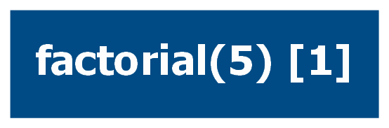
Since the previous implementations are non-recursive, the call graph consists of a single node:
Recursion
After introducing one of the previous definitions of the factorial function, the "recursive form" is usually presented. A recursive function is a function that calls itself. There are multiple types of recursion though, and understanding them may have a huge impact on some programming languages. Before showing what the recursive version of the factorial looks like, it is important to clarify some concepts.
Why Recursion?
Recursion in and of itself is a wide field in computer science that may attract scientists and researchers. However, it is sometimes portrayed as a difficult topic and receives less attention than other techniques.
Although some may avoid recursion altogether, there are clear and noticeable benefits of using recursive functions, such as:
- Declarative style: Recursive functions are written by thinking about what the function does instead of how it does it. The iterative style usually leads the programmer to think about low-level details like indexes and pointers whereas recursion brings the whole problem into mind.
- Simplicity and Readability: Recursive functions can provide a more elegant and concise solution for solving complex problems by breaking them down into simpler subproblems. The recursive approach often closely resembles the problem's definition, making the code more intuitive and easier to understand.
- Divide and Conquer: Recursive functions can leverage the divide and conquer technique, where a problem is divided into smaller subproblems that are solved independently. This approach simplifies the problem-solving process by reducing complex tasks into manageable pieces.
- Code Reusability: Recursive functions are often reusable. Once implemented, they can be called multiple times with different inputs, allowing for efficient and modular code. Recursive functions can be applied to various instances of the same problem, enabling code reuse and promoting good software engineering practices.
- Handling Recursive Structures: Recursive functions are especially useful when dealing with recursive data structures, such as trees or linked lists. The recursive nature of the data can be mirrored in the recursive functions, making it easier to traverse, manipulate, or process such structures.
- Mathematical and Algorithmic Modeling: Many mathematical and algorithmic problems are naturally defined in terms of recursion. Recursive functions provide a natural and direct way to express these problems, making the code more closely aligned with the underlying mathematical or algorithmic concepts.
- Time and Space Optimization: Recursive functions can often lead to more efficient algorithms in terms of time and space complexity. By breaking down a problem into smaller subproblems, recursive functions can avoid unnecessary computations by reusing previously calculated results (memoization) or eliminating redundant iterations.
Direct vs Indirect Recursion
Most commonly, when one says "recursive function", it is meant "direct recursive function", that is, the function calls itself. The other way a function could be recursive is through "indirect recursion" where, instead of calling itself, it calls another function (or chain of functions) that will in turn call the first function.
Different types of direct recursions worth mentioning are:
Based on where the recursive call is done:
- Head Recursion
- Middle Recursion
- Tail Recursion
Based on the number of recursive calls:
- Linear Recursion
- Multi Recursion (also called nonlinear or exponential recursion)
- Tree Recursion (also called bifurcating recursion)
- Nested Recursion
- General Non-Linear Recursion
Based on the number of functions involved:
- Direct Recursion (a single function)
- Indirect Recursion (multiple functions, also called mutual recursion)
Besides the previous classification, all recursive functions must have a termination condition or else they would enter in an infinite loop. Even though recursive functions do not need to be pure (i.e. they do not have side effects), it is common for recursive functions to be pure, this simplifies the interpretation. All the examples in this article are pure functions.
Linear Recursion
Linear recursion refers to functions where there is only one recursive call.
Based on the position of the recursive call it could be further subdivided into:
- Head Recursion: recursive call is the first statement.
- Middle Recursion: there are other statements before and after a recursive call.
- Tail Recursion: recursive call is the last statement.
There is no difference between Middle Recursion and Head Recursion from an efficiency and algorithmic perspective. So no further exploration will not be done on those two.
When a function has more than one recursive call is called Multi Recursion, Nonlinear Recursion or Exponential Recursion. These cases will be covered in a later section.
The following is an example of a middle recursion implementation of the factorial function.
def factorial(n: int) -> int:
    """Middle Recursion implementation of the factorial function"""
    if n == 0:
        return 1
    return n * factorial(n - 1)

assert [factorial(i) for i in range(7)] == [1, 1, 2, 6, 24, 120, 720]
It is middle recursion because the last statement is a multiplication (*) and
not the recursive call itself. Depending on the operation order it could also be
considered head recursion but that difference is not relevant for most contexts.
Another way to better show why this is middle recursion is to use additional variables to store interim results:
def factorial(n: int) -> int:
    """Middle Recursion implementation of the factorial function"""
    if n == 0:
        return 1
    previous_factorial = factorial(n - 1)
    current_factorial = n * previous_factorial
    return current_factorial

assert [factorial(i) for i in range(7)] == [1, 1, 2, 6, 24, 120, 720]
In this more explicit implementation, it is clearer that the last logical
statement is the multiplication n * previous_factorial.
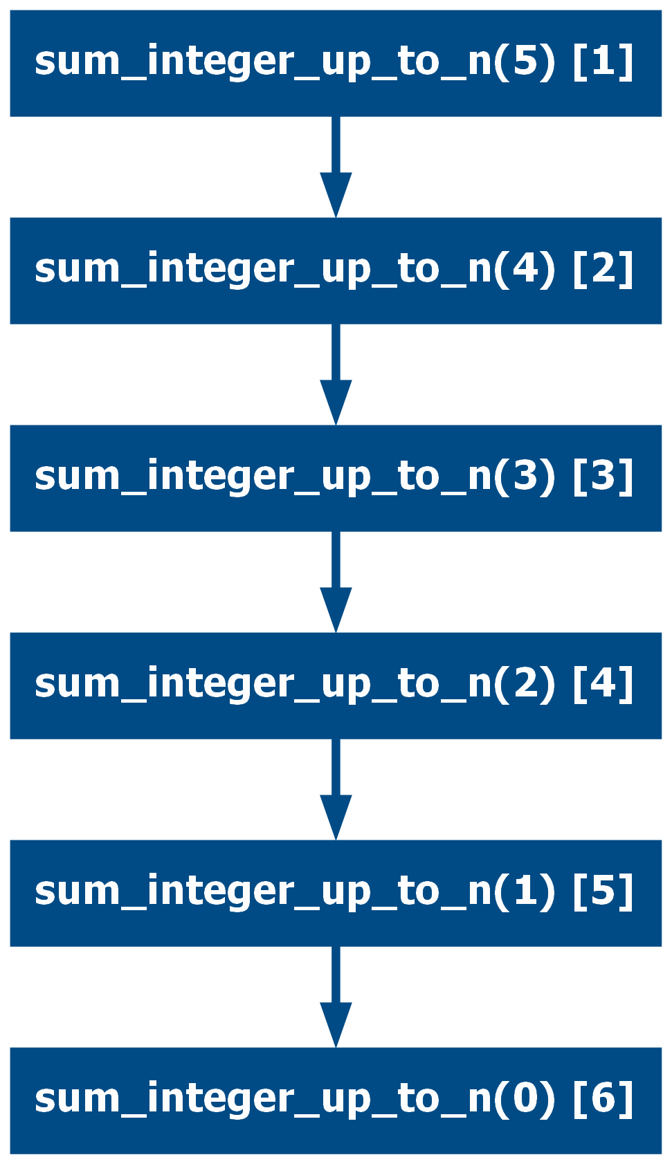
The call graph in the case of linear recursive functions is a series of nodes called sequentially, hence the name:
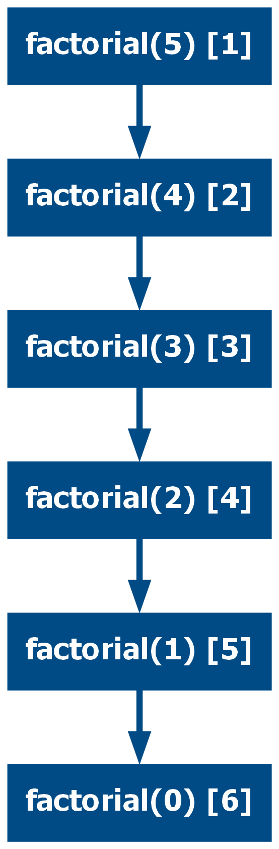
When the last statement is the recursive call, the function is called tail recursion, which will be explored in the next section.
Tail Recursion
Tail recursion is when the return statement of the function is only a recursive call, this means that a function call could be replaced with another function call directly. Some languages (Python is not one of them), use a technique named Tail-Call Optimization, which makes this particular type of recursion very efficient.
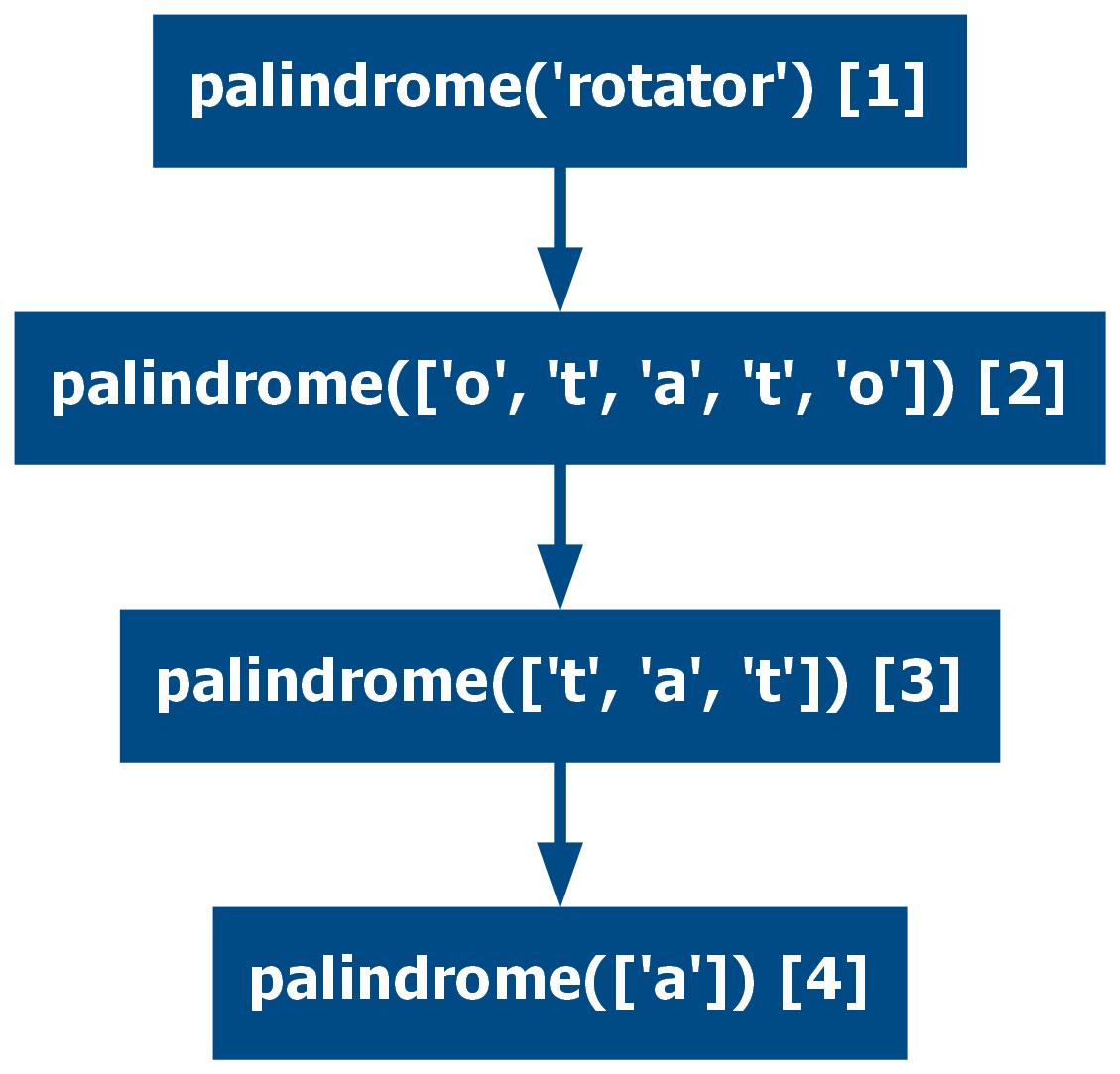
One important clarification is that the return must not be an expression. An
example of a straightforward function that can be implemented in a tail
recursive way is the palindrome function:
def palindrome(string: str) -> bool:
    "Returns True if the given string is a palindrome. Using tail recursion."
    if len(string) < 2:
        return True

    first, *rest, last = string
    if first != last:
        return False
    return palindrome(rest)

assert palindrome("a")
assert palindrome("aa")
assert palindrome("aba")
assert not palindrome("learn")
assert palindrome("rotator")
To better illustrate the fact that the returning statement must be only a
function call, the following implementation is NOT a tail recursive
function because the last statement is not a function call, it is a boolean
expression that requires the function call to be executed before returning. The
reason is the and operator which needs a value. This implementation is
therefore a middle recursion.
def palindrome(string: str) -> bool:
    "Returns True if the given string is a palindrome. Using middle recursion."
    if len(string) < 2:
        return True

    first, *rest, last = string
    return first == last and palindrome(rest)

assert palindrome("a")
assert palindrome("aa")
assert palindrome("aba")
assert not palindrome("learn")
assert palindrome("rotator")
Sometimes a function that is not expressed in tail-call form can be converted to that form. For example the following middle recursive function:
def sum_integer_up_to_n(n: int) -> int:
    """Sums all integers from zero to n. Using middle recursion"""
    if n == 0:
        return 0

    return n + sum_integer_up_to_n(n - 1)

assert sum_integer_up_to_n(1) == 1
assert sum_integer_up_to_n(3) == 6
Can be rewritten into tail-recursive form as:
def sum_integer_up_to_n(n: int, total: int = 0) -> int:
    """Sums all integers from zero to n. Using Tail recursion"""
    if n == 0:
        return total

    return sum_integer_up_to_n(n - 1, total=n + total)

assert sum_integer_up_to_n(1) == 1
assert sum_integer_up_to_n(3) == 6
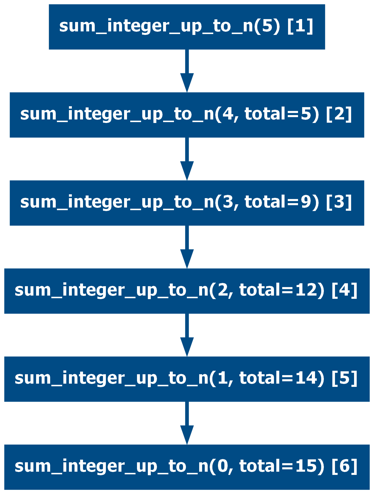
This last version uses an additional parameter to pass the total down the call chain. This compromises readability for performance if the language implements tail-call optimization. This style of programming is widely used in languages like Prolog and some purely-functional languages.
In Python however the extra parameter can be hidden by using default values, this makes the implementation more similar to the original but it is implicitly hiding the way it truly works, which is against many coding styles. Use with caution.
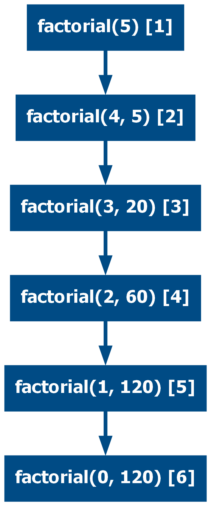
In the same way as sum_integer_up_to_n, the factorial function could be
re-written into a tail recursive form:
def factorial(n: int, result: int = 1) -> int:
    if n == 0:
        return result

    return factorial(n - 1, n * result)

assert [factorial(i) for i in range(7)] == [1, 1, 2, 6, 24, 120, 720]
When comparing head/middle with tail recursion, the way each approach works differs and can be illustrated by inspecting the execution step by step:
# Head/Middle Recursion
factorial(3)
3 * factorial(3 - 1)
3 * factorial(2)
3 * 2 * factorial(2 - 1)
3 * 2 * factorial(1)
3 * 2 * 1 * factorial(1 - 1)
3 * 2 * 1 * factorial(0)
3 * 2 * 1 * 1
6
# Tail Recursion
factorial(3)
factorial(3 - 1, 3 * 1)
factorial(2, 3)
factorial(2 - 1, 3 * 2)
factorial(1, 6)
factorial(1 - 1, 6 * 1)
factorial(0, 6)
6
Multi Recursion
When there is more than one recursive call, a function is said to be multi-recursive. Multi-recursive functions can also be middle/head recursive or tail-recursive. A special case of Multi Recursion is when the recursive call is one of the arguments, in this case, it is referred to as nested recursive.
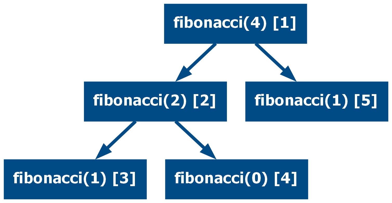
General Non-Linear Recursion
Many functions do not follow a precise pattern and they just use multiple recursive calls as part of their definition. One such example is a function that returns the nth Fibonacci number, to call the function two successive recursive calls are used.
This is the traditional implementation:
def fibonacci(n: int) -> int:
    if n == 0:
        return 0
    if n == 1:
        return 1
    return fibonacci(n - 1) + fibonacci(n - 2)

assert [fibonacci(i) for i in range(7)] == [0, 1, 1, 2, 3, 5, 8]

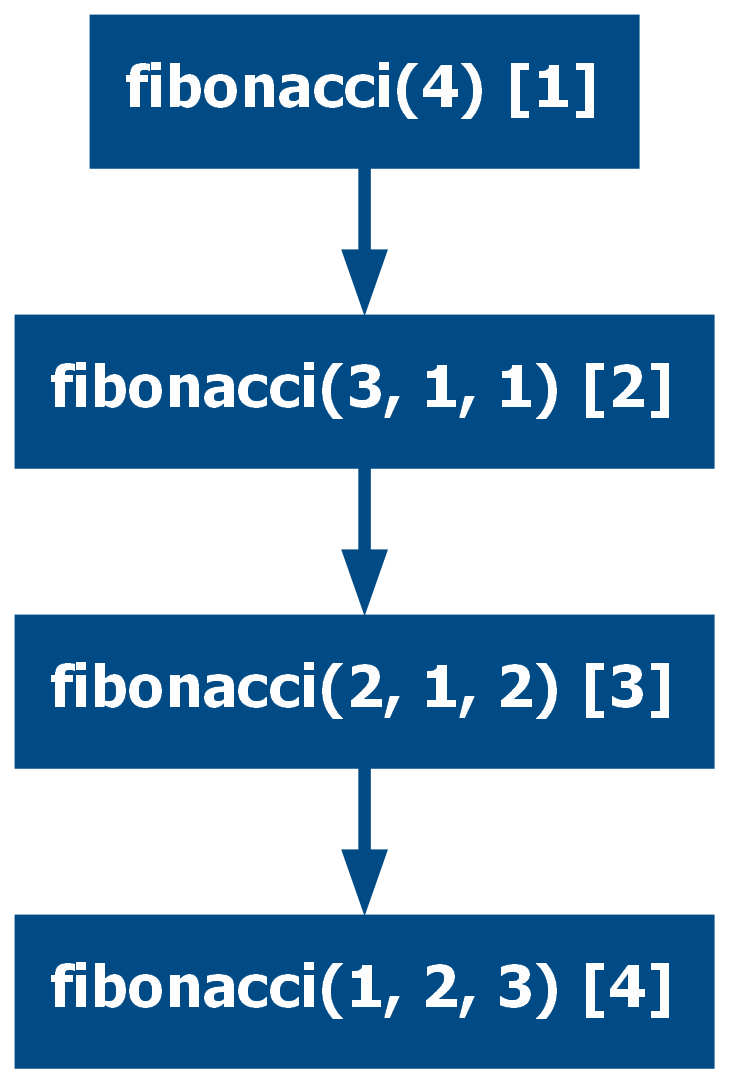
In some cases, multi-recursive functions can be refactored into linear tail recursive functions.
def fibonacci(n: int, partial_result: int = 0, result: int = 1) -> int:
    if n == 0:
        return 0
    if n == 1:
        return result
    return fibonacci(n - 1, result, partial_result + result)

assert [fibonacci(i) for i in range(7)] == [0, 1, 1, 2, 3, 5, 8]
Tree Recursion
In the case of multi-recursive functions, it is possible to construct a tree of the function calls. All multi-recursive functions produce a tree, that being said, in some cases the definition leverages the divide-and-conquer strategy, minimizing the depth of the tree. One example of this is the quicksort algorithm:
from typing import Collection

def quicksort(numbers: Collection[float]) -> list[float]:
    if len(numbers) <= 1:
        return numbers

    first, *rest = numbers

    left = [x for x in rest if x < first]
    right = [x for x in rest if x >= first]
    return quicksort(left) + [first] + quicksort(right)

assert quicksort([2, 4, 3, 5, 0, 1]) == list(range(6))
assert quicksort(list(reversed(range(10)))) == list(range(10))
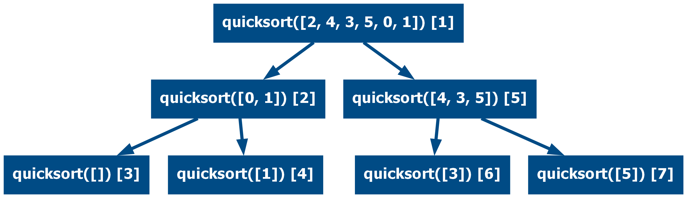
Here the function divides the input into two parts and each recursive call gets one of the parts. This strategy reduces the number of recursive calls by a great amount.
Converting non-tree recursion into tree recursion
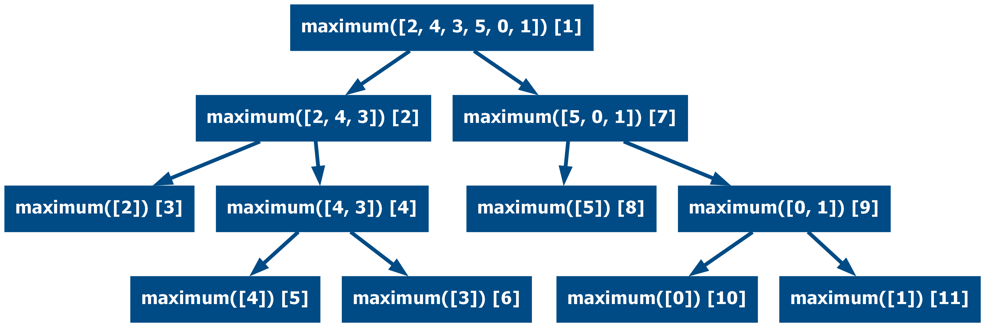
Some functions that are originally linear recursive can be converted into tree recursive to reduce the depth of the recursive stack. This is usually easy on functions that operate on arrays.
Here is a linear recursive implementation of a function that returns the maximum value of a list:
from typing import Iterable

def maximum(numbers: Iterable[float]) -> float:
    first, *rest = numbers
    if not rest:
        return first

    rest_max = maximum(rest)
    return first if first > rest_max else rest_max

assert maximum([2, 4, 3, 5, 0, 1]) == 5
assert maximum(list(range(10))) == 9

This holds even if re-written into a tail-recursive form:
from typing import Optional, Iterable

def maximum(numbers: Iterable[float], max_value: Optional[float] = None) -> float:
    first, *rest = numbers

    if max_value is None or first > max_value:
        max_value = first

    if not rest:
        return max_value

    return maximum(rest, max_value)

assert maximum([2, 4, 3, 5, 0, 1]) == 5

Both implementations will have as many recursive calls as there are elements in the list. A similar approach to the quicksort algorithm can be used to reduce the number of calls, halving the length of the list each time. With this approach, the recursive stack will be shorter.
from typing import Collection

def maximum(numbers: Collection[float]) -> float:
    first, *rest = numbers
    if not rest:
        return first

    middle = len(numbers) // 2
    left_max = maximum(numbers[:middle])
    right_max = maximum(numbers[middle:])
    return left_max if left_max > right_max else right_max

assert maximum([2, 4, 3, 5, 0, 1]) == 5
assert maximum(list(range(10))) == 9
Refactoring functions this way is not always possible, for functions like nth Fibonacci, it is not trivial to use a tree approach that reduces the number of recursive calls. A known solution called Fast Doubling has been discovered. Deriving this implementation requires a lot of effort and mathematical knowledge, such an approach may not apply to other functions.
The Fast Doubling Implementation is as follows:
def fibonacci(n: int) -> int:
    # Fast Doubling Method
    if n == 0:
        return 0
    if n == 1:
        return 1

    is_odd = n % 2
    m = n // 2 + is_odd
    fib_m = fibonacci(m)
    fib_m_1 = fibonacci(m - 1)

    if is_odd:
        return fib_m_1**2 + fib_m**2
    return 2 * fib_m * fib_m_1 + fib_m**2

assert [fibonacci(i) for i in range(7)] == [0, 1, 1, 2, 3, 5, 8]
It is even possible to further reduce the number of recursive calls by converting the multi-recursive function into a linear recursive function by changing its structure to return two values at once:
def fibonacci(n: int) -> int:
    # based on: https://www.nayuki.io/page/fast-fibonacci-algorithms
    def nth_and_nth_plus_one(n: int) -> tuple[int, int]:
        if n == 0:
            return 0, 1

        fib_m, fib_m_1 = nth_and_nth_plus_one(n // 2)
        nth = fib_m * fib_m_1 * 2 - fib_m**2
        nth_plus_one = fib_m**2 + fib_m_1**2

        is_odd = n % 2
        if is_odd:
            nth_plus_two = nth + nth_plus_one
            return nth_plus_one, nth_plus_two
        return nth, nth_plus_one

    nth, _ = nth_and_nth_plus_one(n)
    return nth

assert [fibonacci(i) for i in range(7)] == [0, 1, 1, 2, 3, 5, 8]
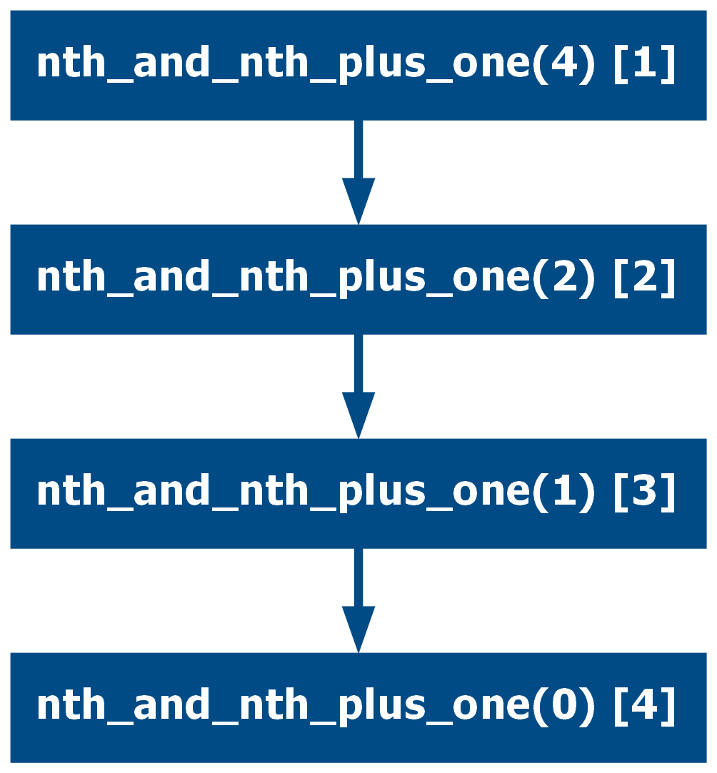
Even though in these examples with fibonacci(4) the difference is not drastic,
the number of total calls in the call graph scales in notoriously different ways
for each implementation, take for example fibonacci(100):
- Typical Multi Recursive Implementation: 1,146,295,688,027,634,168,203 calls ≈ 1 sextillion calls
- Fast Doubles: 163 calls
- Tail Recursive Implementation: 100 calls
- Linear Recursive Implementation: 8 calls
Nested Recursion
One special case of multi-recursion is when the argument of the recursive call is itself a recursive call. This is not usual in software development but could arise in mathematical fields. One example is the Hofstadter G Sequence:
def hofstadter_g(n: int) -> int:
    if n == 0:
        return 0
    return n - hofstadter_g(hofstadter_g(n - 1))

assert [hofstadter_g(i) for i in range(7)] == [0, 1, 1, 2, 3, 3, 4]

Refactoring nested recursion into non-nested multi-recursion or linear recursion is a non-trivial task and sometimes it may be impossible.
Triple Nested Recursion
The level of nesting is not limited to just two calls, the Hofstadter H Sequence has triple nesting recursion for example:
def hofstadter_h(n: int) -> int:
    if n == 0:
        return 0
    return n - hofstadter_h(hofstadter_h(hofstadter_h(n - 1)))

assert [hofstadter_h(i) for i in range(6)] == [0, 1, 1, 2, 3, 4]
Nested Recursion with more than one argument
Some functions can have multiple arguments and be nested recursive. One example is the Ackermann function grows extremely fast due to this nested recursive definition and it is the simplest function proved not to be primitive recursive, meaning that it cannot be expressed in iterative form with for loops.
This function is currently used to test compilers' efficiency at handling really deep recursive functions. This is a case of a nested recursive function that is also tail recursive.
def ackermann(m: int, n: int) -> int:
    if m == 0:
        return n + 1
    if m > 0 and n == 0:
        return ackermann(m - 1, 1)
    return ackermann(m - 1, ackermann(m, n - 1))

assert [ackermann(i, j) for i in range(3) for j in range(3)] == [1, 2, 3, 2, 3, 4, 3, 5, 7]
Indirect Recursion
So far, all the examples showed functions that called themselves, this is direct recursion. An alternative approach is indirect recursion, also known as mutual recursion. In this case, the same categories could be applied (linear, tail, head, nested, etc.), but the recursive call is now to another function, that other function will, in turn, call the original one.
Mutual Linear Recursion
A simple example of mutual linear tail recursion is a set of functions that determines if a number is odd or even:
def is_even(n: int) -> bool:
    if n == 0:
        return True
    return is_odd(n - 1)

def is_odd(n: int) -> bool:
    if n == 0:
        return False
    return is_even(n - 1)

assert [is_even(i) for i in range(6)] == [True, False, True, False, True, False]
assert [is_odd(i) for i in range(6)] == [False, True, False, True, False, True]
Of course, it is also possible to implement a function that computes the same in a non-recursive form. However, this example does not require division or modulo computation, it is much slower for big numbers.
Mutual Multi Recursion
Mutual recursion can also happen in multi-recursive functions. Take the following direct multi-recursive function that computes the nth Lucas number:
def lucas(n: int) -> int:
    if n == 0:
        return 2
    if n == 1:
        return 1
    return lucas(n - 1) + lucas(n - 2)

assert [lucas(i) for i in range(7)] == [2, 1, 3, 4, 7, 11, 18]

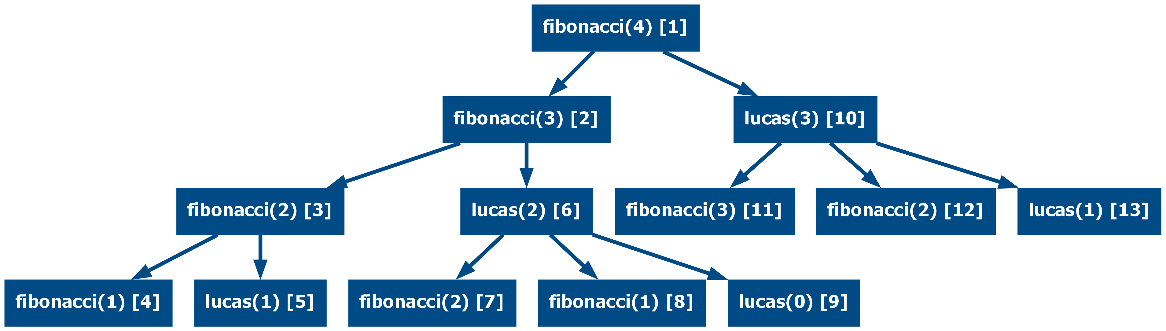
It is possible to write both the Lucas and the Fibonacci functions in a mutual recursive form:
def lucas(n: int) -> int:
    if n == 0:
        return 2
    if n == 1:
        return 1
    return 2 * fibonacci(n) - fibonacci(n - 1) + lucas(n - 2)

def fibonacci(n: int) -> int:
    if n == 0:
        return 0
    if n == 1:
        return 1
    return (fibonacci(n - 1) + lucas(n - 1)) // 2

assert [lucas(i) for i in range(5)] == [2, 1, 3, 4, 7]
assert [fibonacci(i) for i in range(5)] == [0, 1, 1, 2, 3]
This implementation is standalone and does not require any of the two functions to be defined in a direct recursive way. In practical terms, there is no gain as it makes the whole computation slower and less efficient, it is just for demonstration purposes.
Similarly, the sequence defined as the multiplication of the last two terms can be implemented in a direct multi-recursive form:
def multiply_last_two(n: int) -> int:
    if n == 0:
        return 1
    if n == 1:
        return 2
    return multiply_last_two(n - 1) * multiply_last_two(n - 2)

assert [multiply_last_two(i) for i in range(7)] == [1, 2, 2, 4, 8, 32, 256]
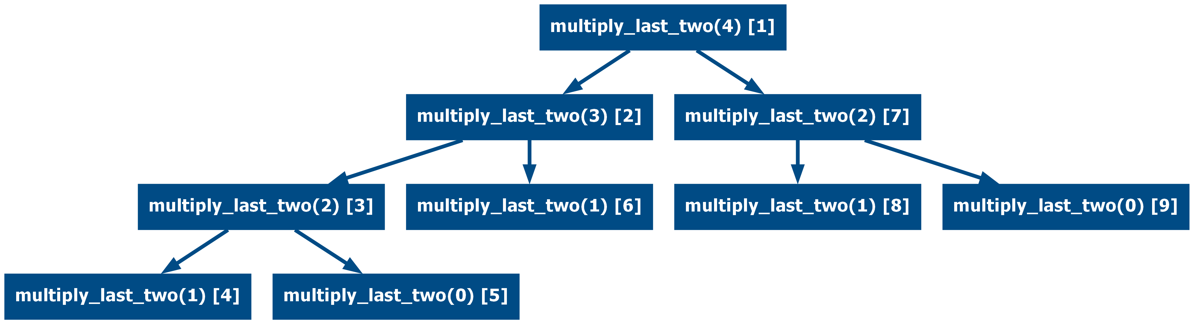
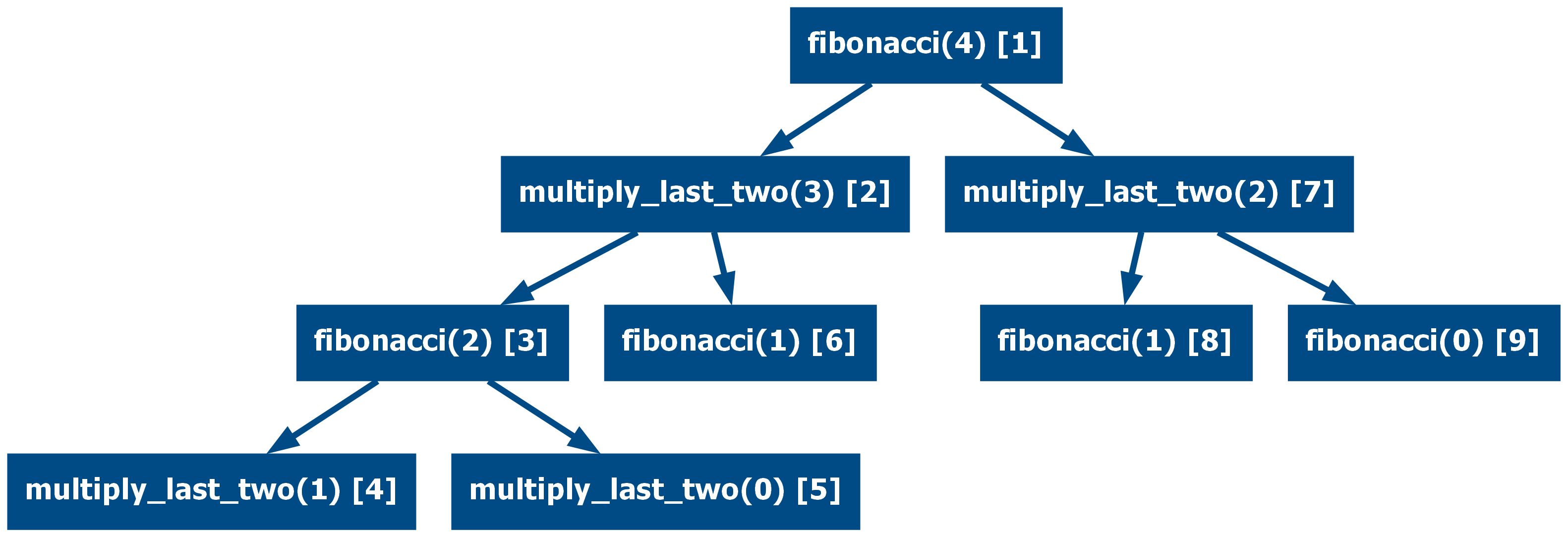
This again can be used to implement the Fibonacci and the multiply last two as mutually recursive functions.
import math

def fibonacci(n: int) -> int:
    if n == 0:
        return 0
    if n == 1:
        return 1
    return int(math.log2(multiply_last_two(n - 1) * multiply_last_two(n - 2)))

def multiply_last_two(n: int) -> int:
    if n == 0:
        return 1
    if n == 1:
        return 2
    return 2 ** (fibonacci(n - 1) + fibonacci(n - 2))

assert [fibonacci(i) for i in range(7)] == [0, 1, 1, 2, 3, 5, 8]
assert [multiply_last_two(i) for i in range(7)] == [1, 2, 2, 4, 8, 32, 256]
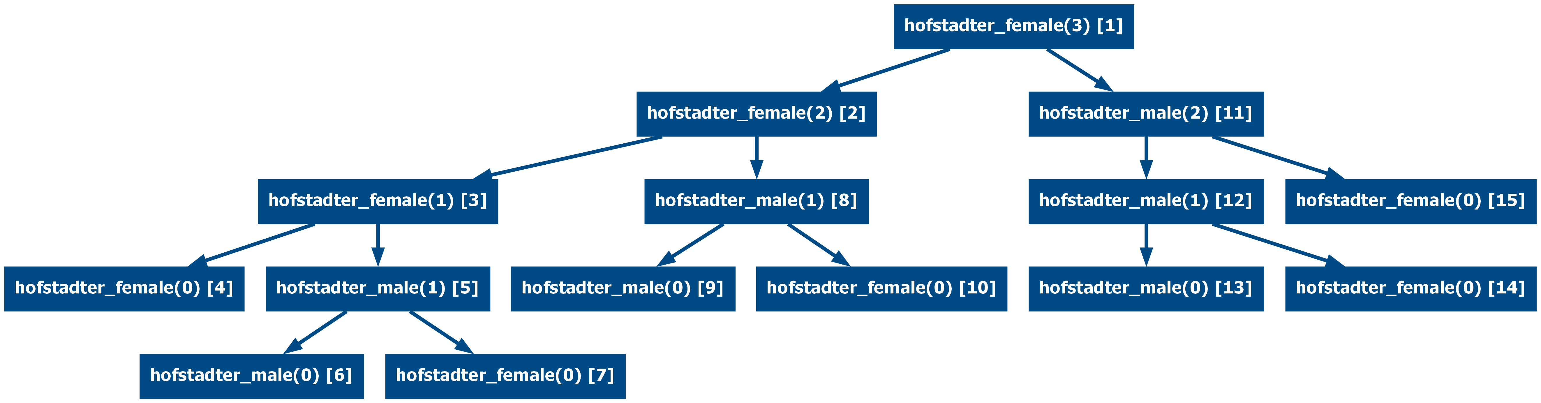
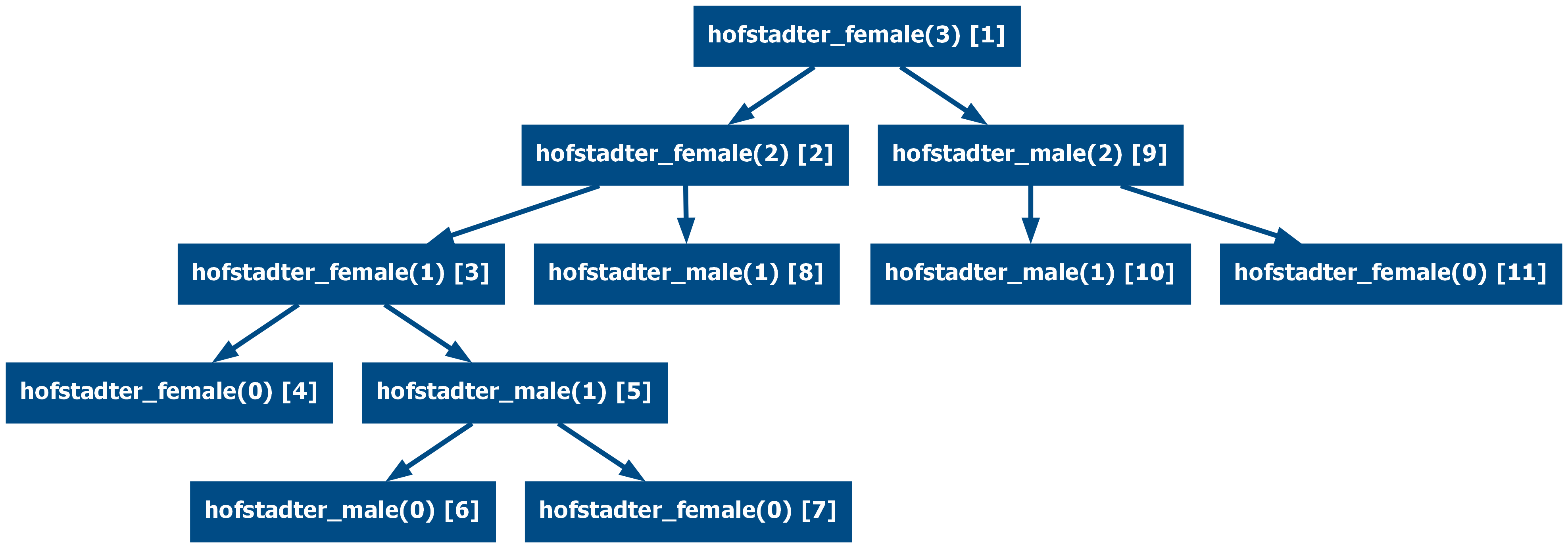
Mutual Nested Recursion
Mutual recursion can also appear in a nested form, as is the case of the Hofstadter Female and Male sequences which are mutually nested recursive.
def hofstadter_female(n: int) -> int:
    if n == 0:
        return 1
    return n - hofstadter_male(hofstadter_female(n - 1))

def hofstadter_male(n: int) -> int:
    if n == 0:
        return 0
    return n - hofstadter_female(hofstadter_male(n - 1))

assert [hofstadter_female(i) for i in range(6)] == [1, 1, 2, 2, 3, 3]
assert [hofstadter_male(i) for i in range(6)] == [0, 0, 1, 2, 2, 3]
Mutual Triple Recursion
Indirect recursion is not limited to only two functions, the following example combines the Lucas, Fibonacci and multiply last two functions in a triple mutual recursive form, where each function uses the other two and itself.
import math

def lucas(n: int) -> int:
    if n == 0:
        return 2
    if n == 1:
        return 1
    return (
        2 * math.log2(multiply_last_two(n - 1) * multiply_last_two(n - 2))
        - fibonacci(n - 1)
        + lucas(n - 2)
    )

def fibonacci(n: int) -> int:
    if n == 0:
        return 0
    if n == 1:
        return 1
    return (fibonacci(n - 1) + lucas(n - 1)) // 2

def multiply_last_two(n: int) -> int:
    if n == 0:
        return 1
    if n == 1:
        return 2
    return 2 ** (1.5 * fibonacci(n - 2) + 0.5 * lucas(n - 2))

assert [lucas(i) for i in range(6)] == [2, 1, 3, 4, 7, 11]
assert [fibonacci(i) for i in range(6)] == [0, 1, 1, 2, 3, 5]
assert [multiply_last_two(i) for i in range(6)] == [1, 2, 2, 4, 8, 32]

Recursion related techniques
Recursion is a wide field, and due to language, compilers and general developer experience limitations, several tools and techniques have been developed to improve recursion support and performance.
Memoization
When dealing with recursive functions, it is important to keep track of the call stack and optimize it to avoid wasting resources. Many recursive functions call themselves multiple times with the same parameters in their call graph, these repeated calls can be cached (assuming the function is pure) to avoid (1) continuing traversing a recursive tree unnecessarily and (2) returning the result in constant time. This technique of caching previously computed results is called memoization.
Memoization is easy to implement in Python, both from scratch and using the standard library.
The from-scratch implementation can be written using decorators:
from functools import wraps
from typing import Callable, TypeVar, ParamSpec

T = TypeVar("T")
P = ParamSpec("P")

def memoize(function: Callable[P, T]) -> Callable[P, T]:
    cache: dict[str, T] = {}

    @wraps(function)
    def wrapper(*args: P.args, **kwargs: P.kwargs) -> T:
        nonlocal cache

        cacheable_args = str(tuple(sorted(args)) + tuple(sorted(kwargs.items())))
        if cacheable_args not in cache:
            cache[cacheable_args] = function(*args, **kwargs)
        return cache[cacheable_args]

    return wrapper
Another possibility is to use the standard library, which has support for
memoization through functools.cache, this function is available in Python 3.9
or later. For older versions, it is also possible to use functools.lru_cache,
which also adds the capability of setting a max limit of cached entries.
Memoization Examples
This section will show what the call graph of the above examples looks like when memoization is applied.
Take for example the following call graph for a multi-recursive implementation
of fibonacci(5):
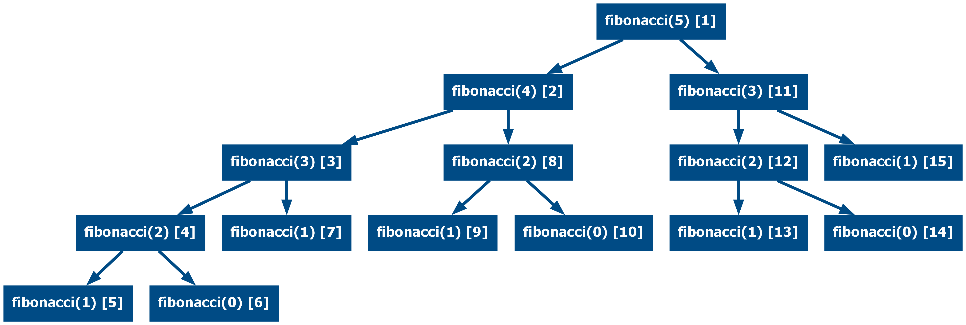
When using memoization the total number of calls is reduced significantly (from 15 calls to 9):

Depending on the implementation, the effect of memoization is similar to linearizing the multi-recursive function, as the tree has much fewer branches while the depth is kept the same.
If considering the Fibonacci Fast Doubles implementation of fibonacci(10):

This can also be reduced (from 15 calls to 11):

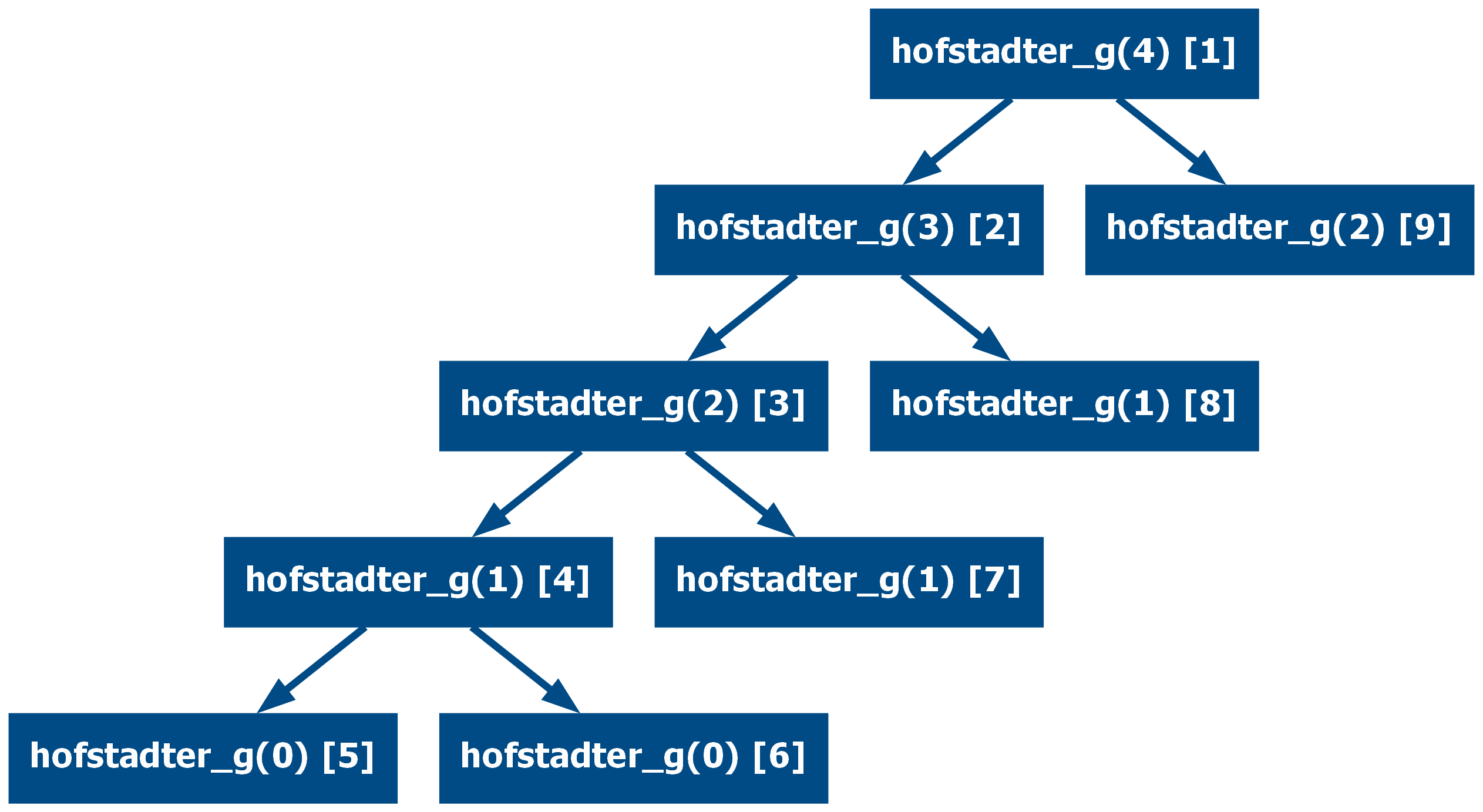
Memoization can also be applied to nested recursive functions such as the
hofstadter_g(4):
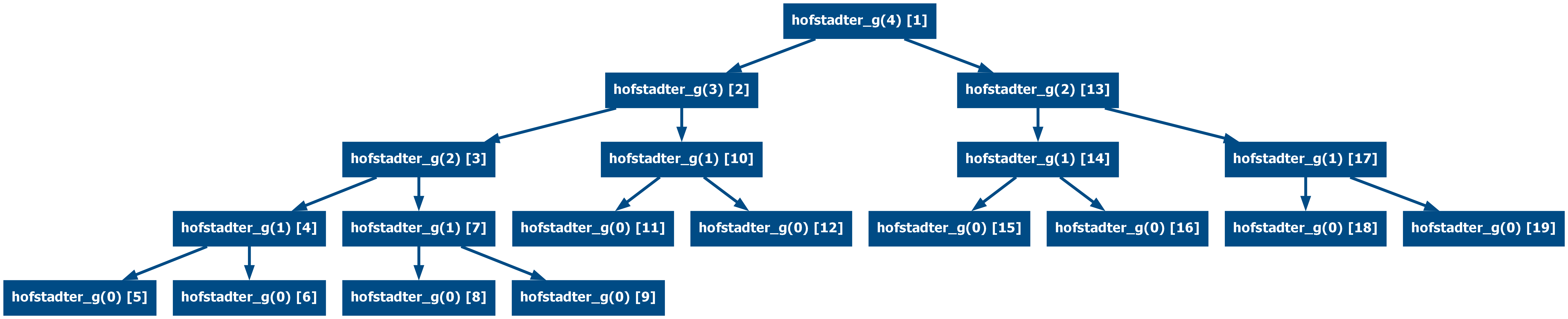
Now memoized (from 19 calls to 9):
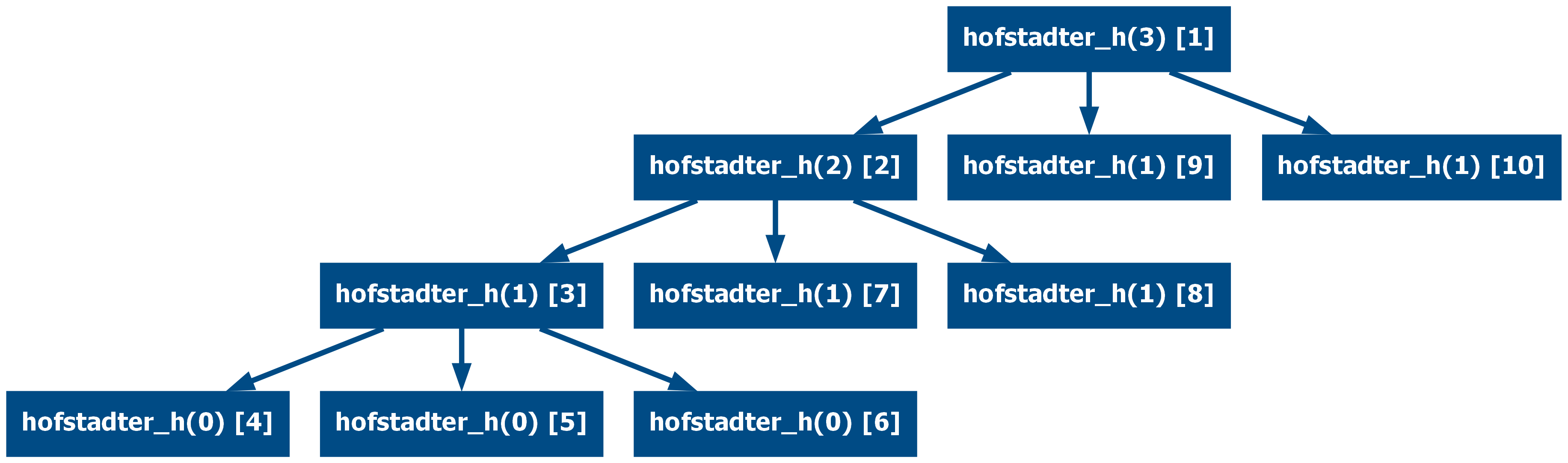
Or deeply nested recursive functions like the hofstadter_h(3):
And now memoized (from 22 to 10 calls)
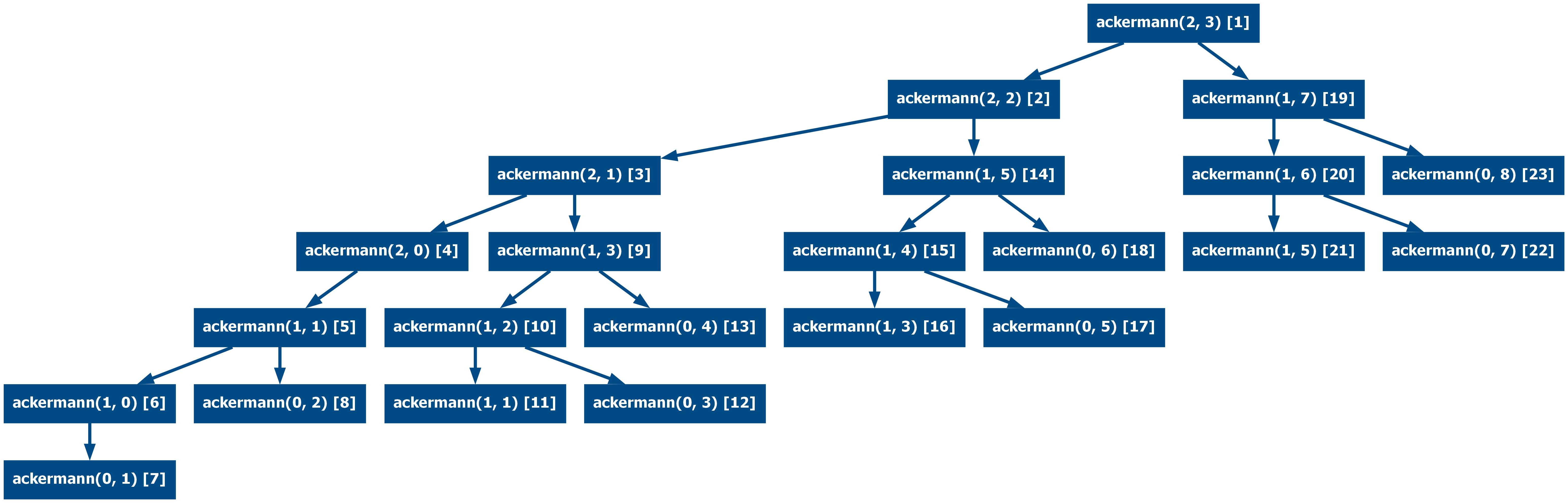
The same applies to more complex functions like the Ackermann function with
Ackermann(2, 3):
And now memoized (from 44 calls to 23):
Memoization can also be used for mutual recursive functions, the following examples show the mutual fibonacci-lucas recursion and the Hofstadter female-male
Multi recursive fibonacci-lucas:
And now memoized (from 26 to 13):
And the hofstadter female-male recursion:
And now memoized (from 15 to 11 calls)
Taking the fibonacci(100) example from the previous section, when
incorporating the memoized approach the results change substantially:
- Typical Multi Recursive Implementation: 1,146,295,688,027,634,168,203 calls ≈ 1 sextillion calls
- Memoized Typical Multi-Recursive Implementation: 199 calls (0.00000000000000002% of the original)
- Fast Doubles: 163 calls
- Tail Recursive Implementation (Memoization has no effect): 100 calls
- Memoized Fast Doubles: 29 calls (17.79% of the original)
- Linear Recursive Implementation (Memoization has no effect): 8 calls
Since the tail recursive and the linear recursive implementation do not have repeated calls, memoization has no effect.
Trampolining
Another restriction that many languages (such as Python) have is call stack overflow, this happens when there are too many recursive calls in the call stack. It is possible with minimal modifications to the original functions to surpass this limitation and make the language treat the recursive function as an iteration and thus bypass the overflow. This technique is called trampoline and requires the function to be implemented in tail-recursive form.
Moreover, the function should defer the evaluation of the tail call by using
an anonymous function (in Python called lambdas). This step is needed to
simulate a lazy evaluation.
The following is an example of how to implement the tail recursive Fibonacci
using trampolining for fibonacci(10000) which would normally cause
RecursionError.
from __future__ import annotations

from typing import TypeVar, Callable, TypeAlias

T = TypeVar("T")
TrampolineFunction: TypeAlias = "Callable[[], T | TrampolineFunction[T]]"

def trampoline(function_or_result: T | TrampolineFunction[T]) -> T:
    if not callable(function_or_result):
        return function_or_result

    while callable(function_or_result):
        function_or_result = function_or_result()

    return function_or_result

def fibonacci(
    n: int, partial_result: int = 0, result: int = 1
) -> int | TrampolineFunction[int]:
    if n == 0:
        return 0
    if n == 1:
        return result

    return lambda: fibonacci(n - 1, result, partial_result + result)

assert str(trampoline(fibonacci(10000))).startswith("3364476487")
This way of programming has several similarities with the continuation passing style since instead of executing the command, the function defers the execution to another function which in the end runs the command. In Object Oriented Programming similar behavior could have been achieved using the Command Pattern.
This particular implementation has a significant drawback, it hinders debugging and makes it less transparent, as can be seen in the run step-by-step example. This is the reason why the author of Python rejected the proposal to incorporate tail call optimization into the language.
The implementation above using lambdas is typical of other languages like
Javascript. In Python, it is possible to implement it in a different way
following Guido's
approach
which makes debugging easier and less cryptic. On the other hand, types become a
bit more convoluted.
from __future__ import annotations

from typing import TypeVar, Callable, TypeAlias, Iterable, cast

T = TypeVar("T")

TrampolineFunction: TypeAlias = "Callable[..., T | TrampolineResult[T] | T]"
TrampolineArgs = Iterable[T]
TrampolineResult: TypeAlias = "tuple[TrampolineFunction[T], TrampolineArgs[T]]"

def trampoline(function: TrampolineFunction[T], args: TrampolineArgs[T]) -> T:
    result = function(*args)

    while isinstance(result, Iterable):
        result = cast("TrampolineResult[T]", result)
        function, args = result
        result = function(*args)

    return result

def fibonacci(
    n: int, partial_result: int = 0, result: int = 1
) -> tuple[TrampolineFunction[int], tuple[int, int, int]] | int:
    if n == 0:
        return 0
    if n == 1:
        return result

    return fibonacci, (n - 1, result, partial_result + result)

assert str(trampoline(fibonacci, (10000,))).startswith("3364476487")
A combination of the previous two approaches can also be achieved by using
partial
evaluation
through functools.partial. This way, the code is simpler and more similar to
what one could find in other languages while still being easy to debug:
from __future__ import annotations

from functools import partial
from typing import TypeVar, Callable, TypeAlias

T = TypeVar("T")
TrampolineFunction: TypeAlias = "Callable[[], T | TrampolineFunction[T]]"

def trampoline(function: T | TrampolineFunction[T]) -> T:
    if not callable(function):
        return function

    while callable(function):
        function = function()

    return function

def fibonacci(
    n: int, partial_result: int = 0, result: int = 1
) -> int | TrampolineFunction[int]:
    if n == 0:
        return 0
    if n == 1:
        return result

    return partial(
        fibonacci, n=n - 1, partial_result=result, result=partial_result + result
    )

assert str(trampoline(fibonacci(10000))).startswith("3364476487")
Trampolines allow to convert of recursive function calls into iterations. There is no built-in support like with the memoized technique and due to technical limitations, it is not possible to implement them as decorators, which would reduce the changes needed on the original function. The different implementations shown should give a grasp of what is possible and how it could be applied to other functions.
It is also possible to modify the default configuration of the interpreter to
allow deeper recursions though. This can be done by setting a higher value to
the
sys.setrecursionlimit.
This method requires however access to the sys module which may not be always
available or editable.
Call-By-Need
Some programming languages execute instructions following a non-strict binding strategy, that is, the parameters of a function are not evaluated before the function is called. One such strategy is called call-by-need, which only evaluates the parameters when needed in the body of the function and caches them in case they are re-used.
When using recursive functions in languages that support call-by-need (like Haskell or R), the execution could be optimized as only a subset of all the recursive calls might be evaluated, thus reducing the cost of recursive functions.
Conclusion
Recursion is a diverse topic that can be used as leverage to overcome challenging problems, improve readability and facilitate the use of recursive data structures. In Python, it is possible to use recursion with some limitations, those could be mitigated by using memoization or trampolines. Other languages may use different strategies such as call-by-need or tail-call optimization.
Every program written in iterative form can be rewritten in recursive form, it is a good exercise to practice and gain intuition about recursion and when it can be applied.
In the end, recursion is another tool, it can be used everywhere but that is not necessarily the best decision always, analyzing the context and the cost-benefits is important.
If recursion is the way to go, aim for tail recursion if possible or to leverage memoization.
Some challenges for the reader to practice recursion:
- Write a function that determines if a number is prime
- Write the addition, multiplication and exponentiation functions
- Write a function that computes a running average of a sequence of numbers